Best-Fit and 3D Comparison
Introduction
Comparing two shapes or two contours to know the gap or distance between them is required when you want to inspect an imported theoretical geometry with the corresponding measured model or when you want to compare two objects at different times (a DTM for instance).
Exercise overview
In this exercise, we will see how to align two objects in the same coordinate system in order to make a 3D comparison.
The process will be as follows:
Reading the theoretical model inside the software (.stl or in case of CAD model, .iges or .step or in case of BIM model, .ifc or rvt).
Reading the "as built" model as a point cloud from the digitization.
Alignment or registration of the scan data on the theoretical model.
Performing distance computation and color texture mapping.
Adding labels.
3D inspection report edition or export.
The files used in this tutorial are HydraulicDam.3dr and TheoriticalModel.stl
The two objects need to be placed in the same coordinate system to be compared. This is why you first have to do a manual alignment or a coarse pre-positioning registration and then use the best fit computation to make the fine registration.
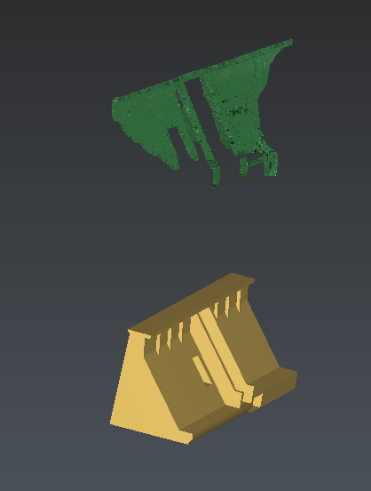 Figure 1: The measured model and the theoretical model are not in the same system
Align the cloud to the model
Open the HydraulicDam.3dr file. It contains a point cloud: the measured model.
Import the TheoriticalModel.stl file. It contains a mesh: the theoretical model.
Select the mesh and launch the N Points Registration command.
This command waits for point couples (departure, target) and computes the transformation that minimizes the distance between each departure point and the corresponding target.
Select these options:
Compute new alignment for the Replay Alignment section
Check Use multiview. it is easier to do the coupling (vertical or horizontal view).
Uncheck all the other options
Click on some couples of points.
Then make a preview, and validate.
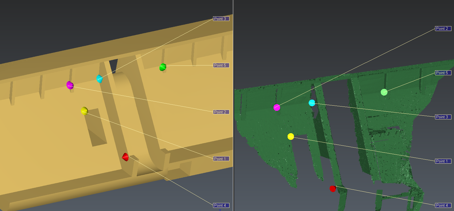 Figure 2: Align the mesh on the point cloud by clicking pairs of points
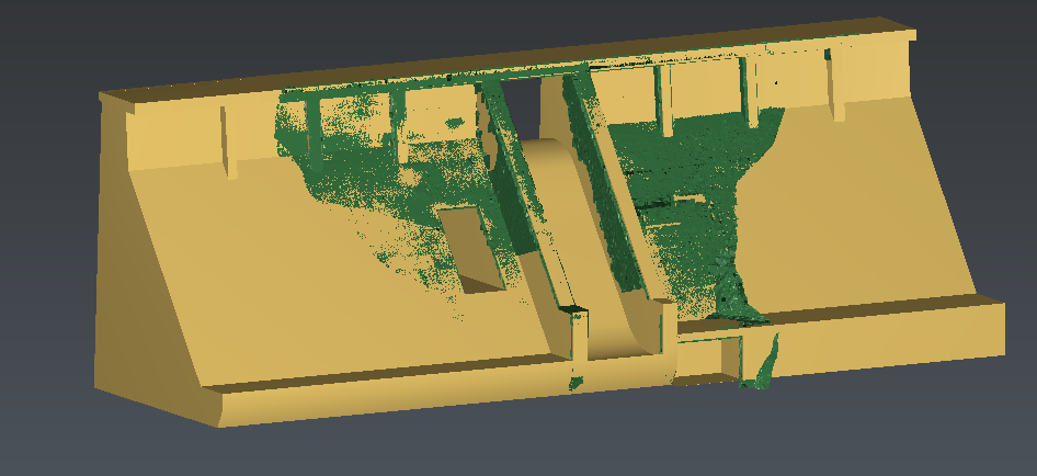 Figure 3: Manual alignment result
Note that clicking on Preview displays some details about the applied transformation. Then, the section of options Define constraints may be useful to preserve the verticality during the movement for example.
Once the two objects are approximately aligned, it is useful to select the two objects and launch the command Best Fit Registration. This command computes the best registration between two objects. Warning! This command can be launched only if the best fit option was not activated in the previous command.
This command analyses the overlap of selected objects to calculate the best fit of these objects. Best-fit means the transformation that minimizes the distance with the other object in a least squares sense.
For the options:
Set Compute new best fit for the Compute method
Set On fixed object (TheoreticalModel) for the Best fit type
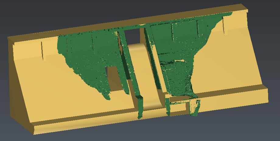 Figure 4: Best-fit registration (the preview displays the transformation information)
Note that a click on Preview displays some details about the applied transformation. Then, the option Define constraints in advanced parameters may be useful to preserve the verticality during the movement for example.
Clean the cloud to remove the aberrant zones
Once the two objects are in the same coordinate system, we can see clearly that the cloud contains some parts that are not present on the model. These zones must be removed because they influence the best fit in a wrong way.
Orient the view like on the next picture (press Y).
Select the point cloud and launch the command Clean / Separate.
Make a contour similar to the one on the picture and press ENTER.
Rotate the view and drag one of the red balls (with the SHIFT key pressed) to take only the aberrant points inside a box.
Click on the bin icon and validate your cleaning with OK.
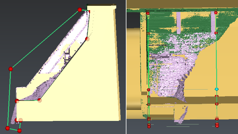 Figure 5: Clean the cloud to remove the aberrant zones
Now, after the cleaning, the best fit must be computed again to obtain a better result.
Select the mesh first, because it must stay immobile, then select the point cloud.
Launch the command Best Fit Registration.
Select the option Compute new best fit.
Click Preview then OK.
Compare and Inspect the two objects
Select the two objects.
Launch Cloud vs Mesh.
The first selected entity is considered as the reference object.
It is possible to choose the object to color (In this case, we want to see if the theoretical model fits with the point cloud, so we will color the theoretical model).
Set the options:
Apply colors on Reference
Check Max distance and set 0.72
Uncheck the other options
Click on Preview. You may have values different from the image below, depending on cleaned points.
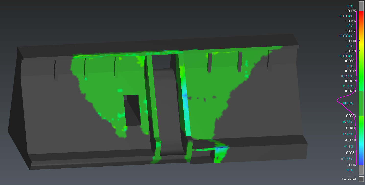 Figure 6: Color map applied on the mesh to see the deviations
Edit Color button opens a dialog box where you can edit the color map. The color map is defined thanks to a tolerance preset where you can modify:
Max and min values which correspond to the minimum and maximum point distance.
Thresholds of each range.
Colors of each range.
Display of the distribution graphic.
The unit.
Note that other options are available to save your inspection parameters for further use. You can access and modify the deviation map when you want from the command Edit Colors.
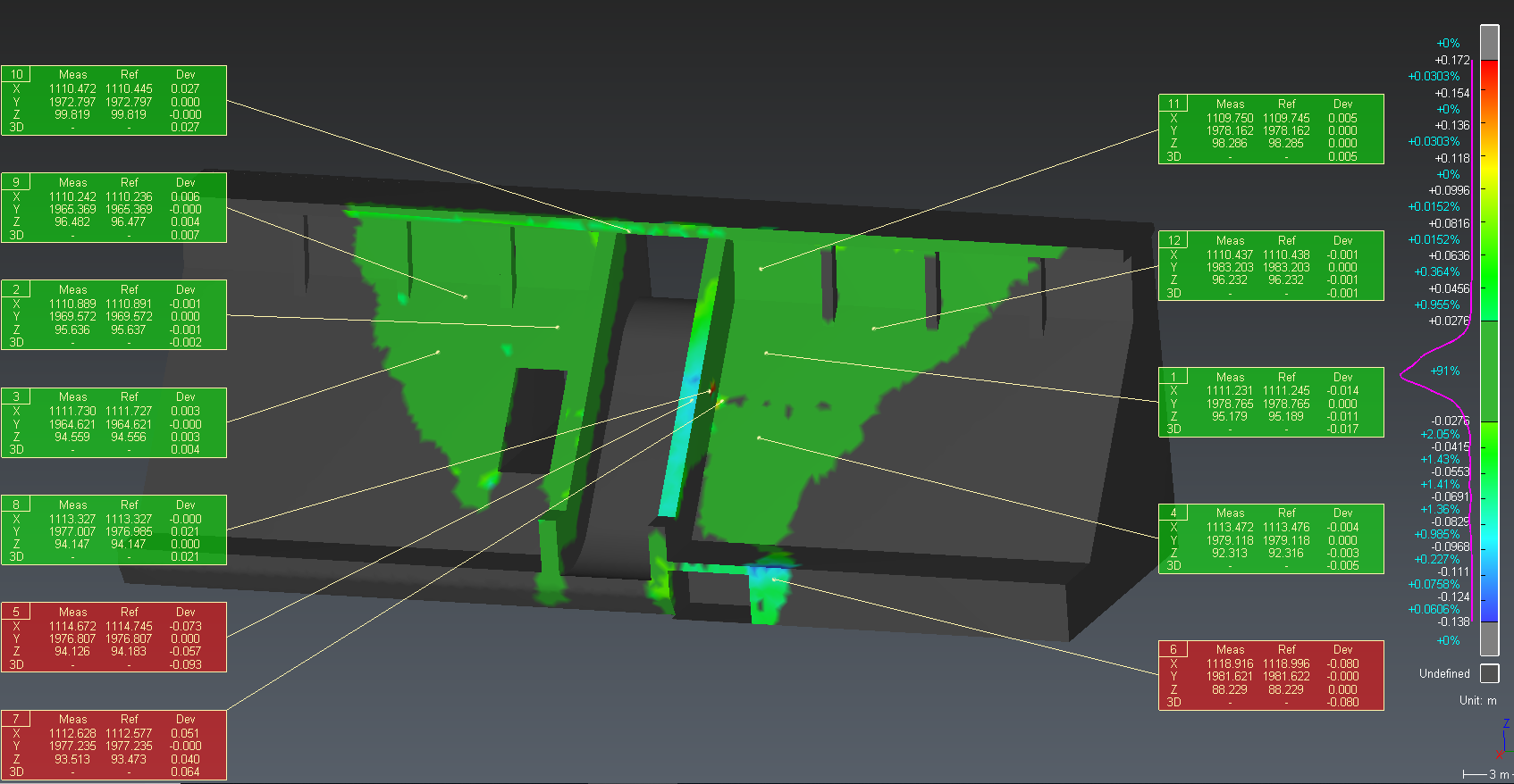
Add labels
To add labels, launch Measure Deviation command and then click on the colored object.
The system searches the reference coordinates, the measured coordinates and the 3D distances. This information of coordinates and distances are completed by the tolerance, label number and comment that you can change into the command.
Set the options:
The max value of the color scale for Tol +, here 0.175
The min value of the color scale for Tol -, here -0.116
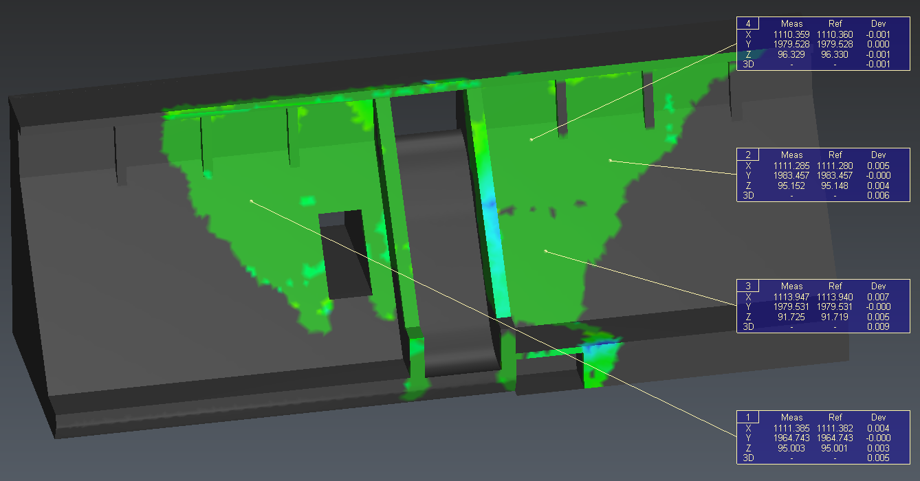 Figure 7: Add labels on specific points
If you want to modify several labels together, for example to set a new tolerance or comment, then select the labels and launch again the command Edit Label.
A click on a label activates the manual shifting of the label.
Edit the aspect of the labels
Launch Label settings to set labels visual properties. You can modify the aspect of the labels: size, color, layout…
Create a report
A report data has been added to the treeview. Orient the 3D scene to show main defects. Then, click on the magnifying glass, corresponding to the report data object which is in the Compare Inspect folder, and update the view. This view will be available within the report editor.
Launch Report Editor and edit your report. For instance:
Remove the cover chapter (refer to Chapters panel).
Remove header and footer (refer to Options panel).
Modify the layout (landscape orientation).
Scene ratio to 5 / 2.
Label size into Minimum
Align the table to the center.
Finally, click on To PDF to generate the report. You can also export the table to a .csv file using the Data panel or the button To CSV.
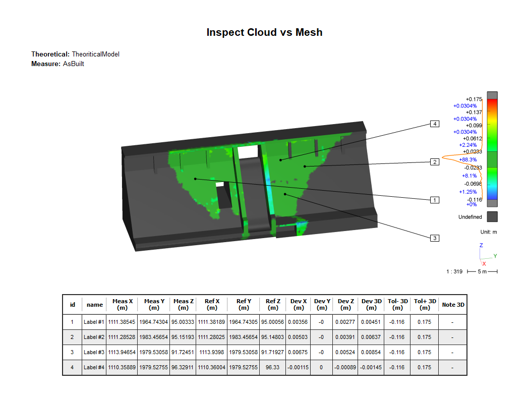 Figure 8: Export the results or/and print a complete report