Differential Settlements
![]()
This command allows you to compute differential settlements of a tank using points around the bottom plate circumference with the method described in API 653 appendix B.
You can enter this command in 3 different ways:
without selection: in this case you will be asked to import an ASCII file containing 3D coordinates of points to be used
with selected points: in this case the selected points will be used
with a selected polyline: in this case the polyline is supposed to represent the bottom plate circumference and you will be able to extract points from it. The command Best Cylinder must have been launched previously
The command Separate Shell can help you to extract the polyline on the bottom plate circumference.
|
|
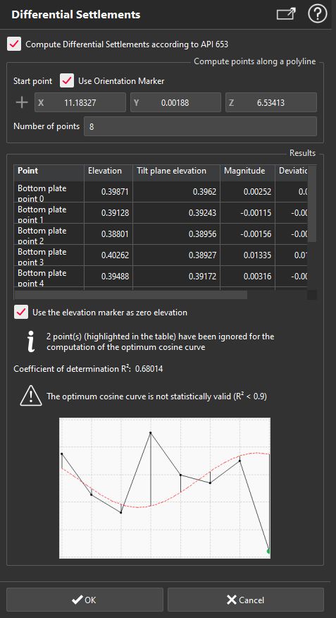
Compute Differential Settlements according to API 653 This option is used to force using more than 7 points, and allows to remove the two worst points for the best cosine computation. Compute points along a polyline (only if you enter with a selected line) In this part you can extract points on the selected line to compute differential settlement. If you check Use Orientation Marker, the first extracted point will be the projection of the reference point of the project on the polyline. Otherwise, you can use the Then you can choose the number of points to extract and to use for calculation. According to API 653 appendix B, points around the circumference are used to compute a best cosine curve representing the tilt plane of the bottom plate. Then for each point, different values are computed and displayed:
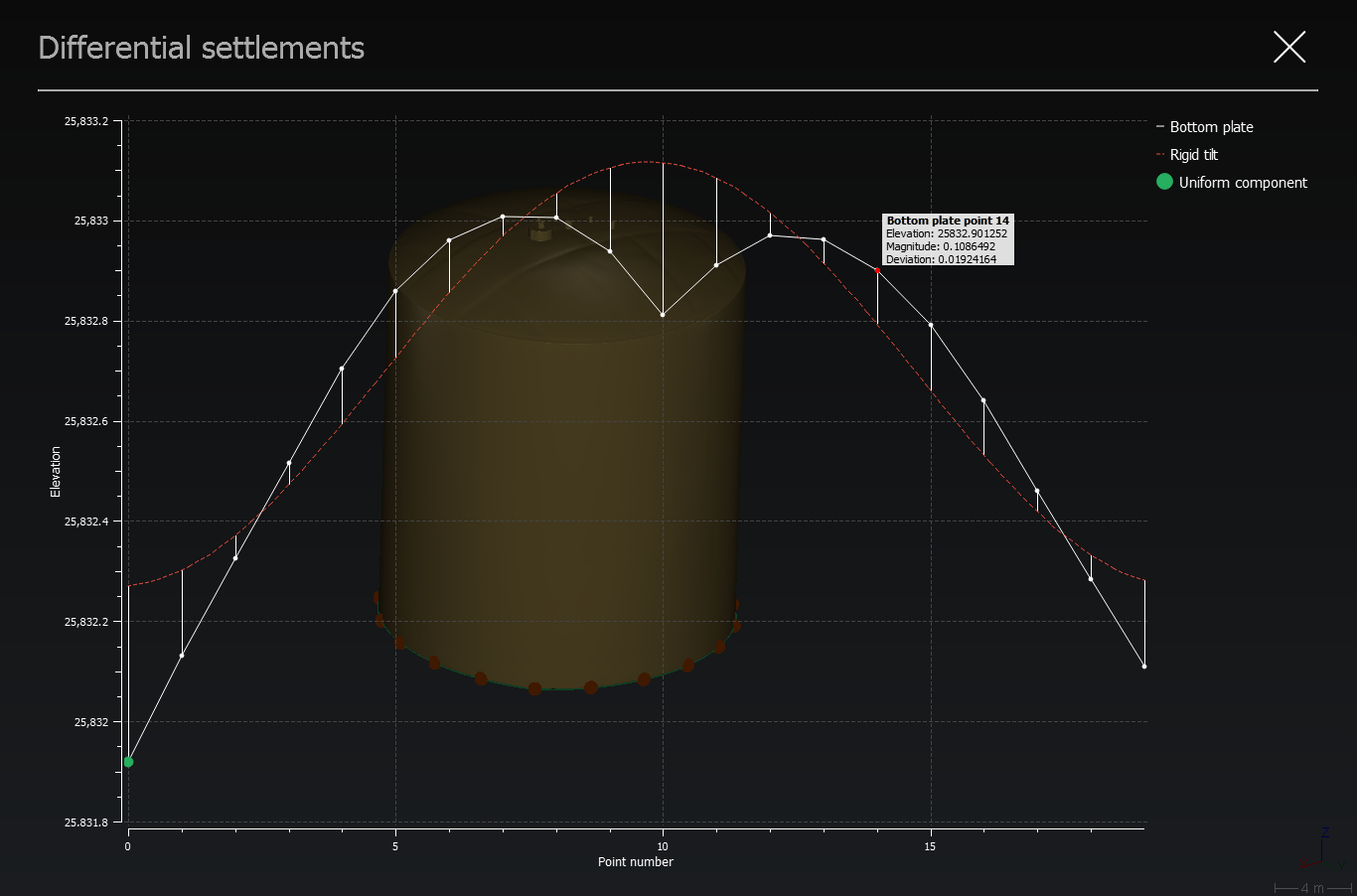
It is also possible to Use Elevation Marker as zero altitude. In this case, the altitude of each point will not be its Z coordinate, but its Z coordinate minus Z coordinate of elevation marker defined for the project. The results are shown in a table and in a 2D plot. Abscissa is the index of the point, and ordinate is the elevation of each point. Elevations are represented by the back plot with black points. The tilt plane (best cosine) is represented by the red plot. Magnitude values are represented by black vertical segments. The computation of the best cosine curve is considered valid only if the coefficient of determination R² is greater than 0.9. To improve the R² value, API 653 standard allows to remove the 2 worst points for computation. In this case a message is displayed and the 2 worst points are underlined in yellow. |
Tip & Trick
By clicking on the 2D plot you can enlarge it over the 3D scene, and then use the cursor to see all the values linked to a point:
Create a report
This command automatically creates reporting data ![]() in your document. This object stores your results so as to create a report later.
in your document. This object stores your results so as to create a report later.
From the treeview click on the magnifier icon![]() to launch the report editor (or launch Report Editor). Then, each object
to launch the report editor (or launch Report Editor). Then, each object ![]() stands for a chapter which can be added to your report.
stands for a chapter which can be added to your report.
Refer to Reporting to learn how to customize your report.