Open the file

Prepare, Define positions and Compute Profiles

Note the smooth/flat color of input objects will be used for new computed objects. It is possible to change this color later by exiting and editing the project. You can click Previous or Next to navigate through the steps of the workflow.

In the first step, Prepare:

1. make sure the axis is oriented correctly. In case of a wrong orientation, you can directly reverse it thanks to the button.

2. define how the positions will be computed (2D or 3D Curvilinear distances). That is to say along the axis or along the projected axis. Set 3D.

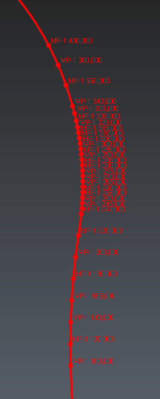
3. define how the positions will be described (Offset and Prefix). Set the offset (1000 m) i.e. the position of the first point of the axis, and set the prefix (MP-).

4. define how the cutting planes will be oriented (Vertical or Locally perpendicular). Set Locally perpendicular: thus the profiles will always be perpendicular to the axis slope.

In the second step, Define Positions, insert the positions defining where profiles have to be computed:

1. insert Regular positions every 20 meters in a Custom range from 1100m to 1400m.

2. insert Regular positions every 5 meters in a Custom range from 1240m to 1320m. Duplicates will not be inserted into the section list.

3. insert other positions thanks to the List of values: 1326 and 1333m.

Positions

In the third step, Compute Profiles, simply compute the profiles and select a display layout. The option Max distance is mainly suitable for road projects to limit the profile extension on its sides.

Compare Inspect the profiles

By default, all deviations will be computed but will be displayed according to the current zoom factor. If you want to fully manage what will be printed, we advise to filter the deviations:

• Use Remove points distant of more/less than to filter out the very high and very low deviations: keep deviations between 0.01m and 0.75m.

• Use Ignore the road to filter out the deviation under an elevation (to give relatively to the axis point): set -2m.

• Activate Compare with regular step either according to a distance along the profile or according to an angle around the axis point: set 15°.

If you are using Profile 2D Inspection, a direction is required to compute and sign the deviations. In that case, Ignore the road is not available and Compare with regular step is only pertinent according to a distance perpendicular to the direction.

When computed, you can click edit color. Not only to edit the color scale but also to manage the quotations texts (unit, number of decimals, magnification of pegs and extreme values):

• keep the default colors and thresholds.

• set the unit to cm.

• do not apply a magnification (1).

• highlight extreme values.

• reduce the number of decimal to 0.

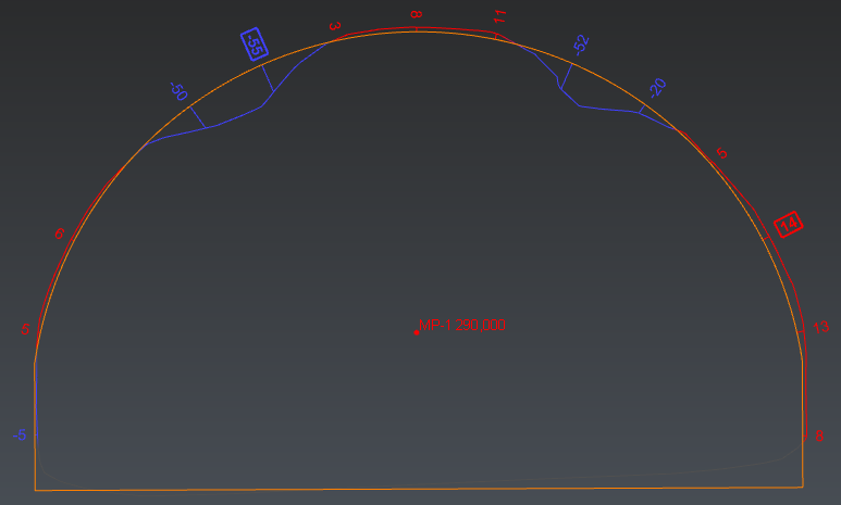MP-1290

Compute the over/under volumes

This optional step is only available in Profile 3D Inspection with meshes. It is strongly advised to use this command with a complete modeling of the two meshes: no sparse triangles, as few holes and as few spikes as possible to generate workable sections.

You can compute overbreak and underbreak volumes between 2 meshes. Only the selected range will be computed and the volume will be divided into slices with 2 drawn profiles at their extremities.

Select the range thanks to the list of positions defined previously (1100-1200m) and adjust the Step to 0.5m that is to say to add intermediate computation profiles. Basically, the computation time will depend on the number of profiles calculated. But the more detailed the mesh is, the lower the step should be. Note a noisy model will create virtual volumes, whatever the step value, since over and under volumes don't eliminate themselves. The method used to compute the volumes is the interpolation between cross sections.

Both meshes are entirely compared to display a 3D mesh colored with two colors: red for overbreak areas and blue for underbreak areas (click edit color to change them). This mesh can be unrolled later.

Export the profiles

In the last workflow step, you can send or export the profiles to AutoCAD or BricsCAD. When you exit the workflow, data are also created to fill a report (refer to the section "Reporting").

Choose the layout among line, column, grid or single. Then select the components to export:

Note the number of decimals of Name and Coordinates can be set here, but the number of decimals for quotations has to be set at the Compare inspect step.

Click the DXF button to generate a DXF file. Otherwise, open a document inside AutoCAD or BricsCAD then click Send to and choose the server.

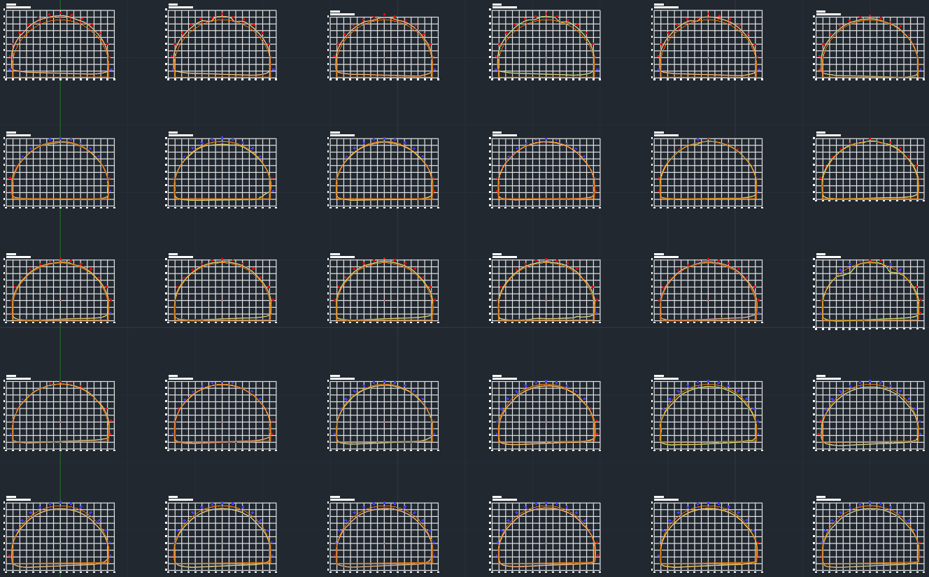Send to (Grid layout)

Creating a 2D inspection map

If Volumes over/under has been computed and if the axis is located at the object center line, it is possible to create a 2D inspection map of the overbreaks and underbreaks.

Select the corresponding colored mesh, the axis and the measured sections MP-1100 and MP-1200. Show only these items using the Contextual menu for instance. Optionally, you can isolate the part between MP-1100 and MP-1200: copy-paste the mesh, select both sections and the pasted mesh and launch Cut Mesh (if you modify the original, it will disappear from previous reports generated).

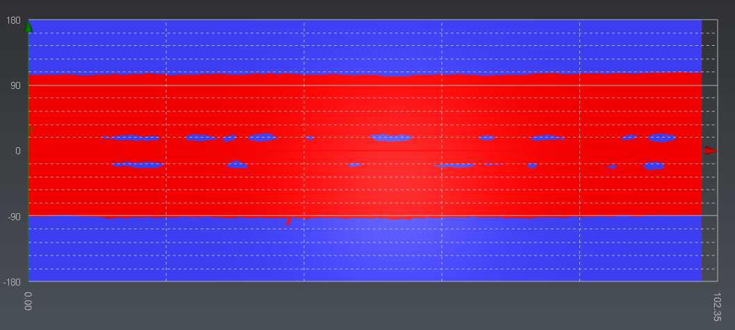
With the mesh and the axis selected, launch the command Unroll around Axis:

• Choose the option 2D.

• Set unit of grid rows to Angle.

• The cutting line is automatically set under the axis.

• Click on Preview to see the result.

• You can display a grid over the map using the bulb. Change the Unit of grid rows to angle.

• You can export a picture of the current scene by clicking on the Export a picture button.

• If you click on OK you will create this 2D map and the grid in the scene.

Reporting

Now, two report data objects have been added to the project: one corresponding to the profiles and the volumes, and one to the unroll. Open the menu Report. Three chapters have been added to the report: a cover page and one chapter per report data object. These chapters are generated thanks to templates assigned to the report data categories. You may want to customize them, for instance:

• Activate the Live Preview to visualize what will be generated according to the defined templates. Undock this window.

• First, define the global layout. Layout settings are common to all chapters. Choose an A4 Portrait layout with headers and footers Not on first chapter. Reduce also the number of decimals.

• Select the cover page and add a title. Use the text toolbar to write it in an appropriate style. You can move the title to the middle of the page by adding some lines. Drag and drop an automatic field (for instance, the date) from the Data panel.

• Sort the chapters as you wish (do a drag and drop).

• Select the Unroll chapter:

  • In the header, add a text area containing the chapter title (use the automatic field because the header is common to all chapters).

  • In the footer, add the page number and the page count.

  • In the body, select the scene to increase the ratio and to modify the scale. Remove the empty item.

• Select the Profile 3D Inspection chapter:

  • Align center the tables.

  • Hide the coordinate system (CS) from the profiles view.

  • In the last table about Detailed volumes, hide the column Volume over and Volume under. Note the last column Opened section indicates the sections which are inaccurate due to holes.

• Finally, press To PDF to generate the report in .pdf.